Note
Go to the end to download the full example code.
Basic pulsar analysis using Fermi-LAT data#
This example shows how to produce the phaseogram of the Crab pulsar, compute the statistics of its peaks, search for pulsations, fit the pulse profile and study the evolution of the signal with time and energy.
It uses about 10 years of public Fermi-LAT observations of the Crab pulsar (100 MeV - 1 GeV), for which the pulsar phases were already computed.
13 import matplotlib.pyplot as plt
14 import numpy as np
15 from astropy.io import fits
16
17 import ptiming_ana
18 from ptiming_ana.phaseogram import PulsarAnalysis
ptiming_ana reports the progress and the results of the analysis through
the Python logging system. This shows the messages in the terminal/notebook:
26 ptiming_ana.setup_logging()
<Logger ptiming_ana (INFO)>
Create the PulsarAnalysis object and settings#
All the settings of the analysis can be read from a configuration file:
35 h = PulsarAnalysis()
36 h.set_config("./example_data/config_tutorial.yaml")
Alternatively we can set the parameters directly#
The phase regions used to compute the statistics of the peaks (P1 and P2) and to estimate the background, the binning of the phaseogram, the time interval used to follow the evolution of the signal, the model used to fit the pulse profile and the energy binning:
47 h = PulsarAnalysis()
48 h.setBackgroundLimits([0.52, 0.87])
49 h.setPeaklimits(
50     P1_limits=[0, 0.026, 0.983, 1], P2_limits=[0.377, 0.422], P3_limits=None
51 )
52 h.setBinning(50, xmin=0, xmax=1)
53 h.setTimeInterval(tint=3600 * 24)
54 h.setFittingParams(model="dgaussian", binned=True)
55 h.setEnergybinning(
56     np.geomspace(0.1 / 1e3, 1 / 1e3, 3), do_diff=True, do_integral=False
57 )  # in TeV
Extracting phases, times and energies from file and give them to the object#
For Fermi data there is a class to read these lists and use them in the main object.
66 h.setFermiInputFile("./example_data/merged2_pulsar.fits")
But in general we can read our file (FITS, DL2, DL3…) and extract phases, times and energies as lists and read them as follows:
73 with fits.open("./example_data/merged2_pulsar.fits") as f:
74     fits_table = f[1].data
75     times = np.array(fits_table["BARYCENTRIC_TIME"], dtype=float)
76     phases = np.array(fits_table["PULSE_PHASE"], dtype=float)
77     energies = np.array(fits_table["ENERGY"], dtype=float)  # in MeV
78
79 h.setListsInput(phases, times, energies / 1e6, tel="fermi", energy_units="TeV")
Run the code#
86 h.run()
2026-10-15 10:44:03 INFO   [ptiming_ana.phaseogram.pulsar_analysis] Initializing...
2026-10-15 10:44:03 INFO   [ptiming_ana.phaseogram.read_events] Finishing reading. Total time is 8342.590926586941 h
2026-10-15 10:44:03 INFO   [ptiming_ana.phaseogram.pulsar_analysis] Calculating statistics every 1440.0 minutes...
2026-10-15 10:44:09 INFO   [ptiming_ana.phaseogram.pulsar_analysis] Fitting the data to the given model...
2026-10-15 10:44:09 INFO   [ptiming_ana.phaseogram.pulsar_analysis] Fit model: dgaussian
2026-10-15 10:44:09 INFO   [ptiming_ana.phaseogram.pulsar_analysis] Binned fitting: True
2026-10-15 10:44:10 INFO   [ptiming_ana.phaseogram.pulsar_analysis] Performing energy-dependent analysis...
2026-10-15 10:44:10 INFO   [ptiming_ana.phaseogram.penergy_analysis] Creating object in energy range (TeV):0.00-0.00
2026-10-15 10:44:10 INFO   [ptiming_ana.phaseogram.penergy_analysis] Calculating statistics...
2026-10-15 10:44:12 INFO   [ptiming_ana.phaseogram.pulsar_analysis] Fitting the data to the given model...
2026-10-15 10:44:12 INFO   [ptiming_ana.phaseogram.pulsar_analysis] Fit model: dgaussian
2026-10-15 10:44:12 INFO   [ptiming_ana.phaseogram.pulsar_analysis] Binned fitting: True
2026-10-15 10:44:12 INFO   [ptiming_ana.phaseogram.penergy_analysis] Creating object in energy range (TeV):0.00-0.00
2026-10-15 10:44:12 INFO   [ptiming_ana.phaseogram.penergy_analysis] Calculating statistics...
2026-10-15 10:44:15 INFO   [ptiming_ana.phaseogram.pulsar_analysis] Fitting the data to the given model...
2026-10-15 10:44:15 INFO   [ptiming_ana.phaseogram.pulsar_analysis] Fit model: dgaussian
2026-10-15 10:44:15 INFO   [ptiming_ana.phaseogram.pulsar_analysis] Binned fitting: True
2026-10-15 10:44:15 INFO   [ptiming_ana.phaseogram.pulsar_analysis] FINISHED. Producing general results...
Show the results#
Overall results#
96 phaseogram = h.draw_phaseogram(phase_limits=[0, 2], colorhist="xkcd:baby blue")
97 plt.tight_layout()
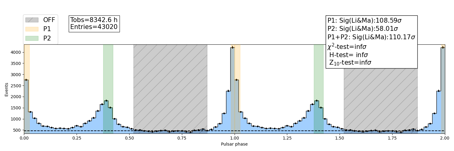
Statistics of the peaks (Li&Ma significance, number of excess events…) and results of the periodicity tests (\(\chi^2\), \(Z^2_{10}\) and H tests):
2026-10-15 10:44:15 INFO   [ptiming_ana.phaseogram.pulsar_analysis] RESULTS FOR THE PEAK STATISTICS:
                       P1           P2         P1+P2
Significance   108.591359    58.006568    110.165719
Nex           5959.237143  2677.271429   8636.508571
Nex_error       84.220286    62.208240    105.936656
Number        6969.000000  3734.000000  10703.000000
noff          1009.762857  1056.728571   2066.491429
sign_t_ratio     1.188899     0.635077      1.206135
s/n ratio      187.534413    82.358927    189.985915
2026-10-15 10:44:15 INFO   [ptiming_ana.phaseogram.pulsar_analysis] P1/P2 ratio=2.23 +/- 0.06
2026-10-15 10:44:15 INFO   [ptiming_ana.phaseogram.pulsar_analysis] RESULTS FOR THE PERIODICITY SEARCH:
                    Chi_square_test       Zn_test        H_test
Statistic              26977.433752  25612.347810  27915.973962
p-value                    0.000000      0.000000      0.000000
Number of $\sigma$       163.171174    159.548517    149.027746
106 peak_statistics
Result of the fitting#
117 print(h.fit_model)
dgaussian
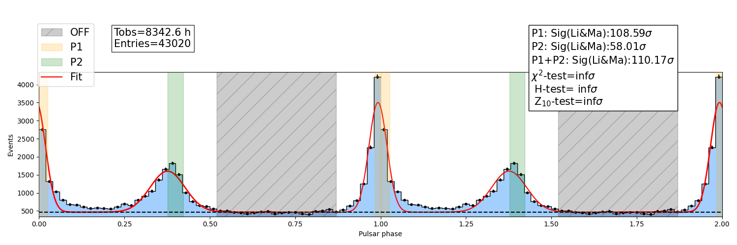
120 fit_result = h.show_fit_results()
121 fit_result
2026-10-15 10:44:15 INFO   [ptiming_ana.phaseogram.pulsar_analysis] FITTING RESULTS:
      Name       Value      Error
0       mu    0.992423   0.001566
1    sigma    0.026305   0.001470
2     mu_2    1.376341   0.004402
3  sigma_2    0.050986   0.004192
4        A  466.437500   0.000000
5        B  200.237289  10.903034
6        C  145.133366  11.041673
124 phaseogram = h.draw_phaseogram(
125     phase_limits=[0, 2], colorhist="xkcd:baby blue", fit=True
126 )
127 plt.tight_layout()
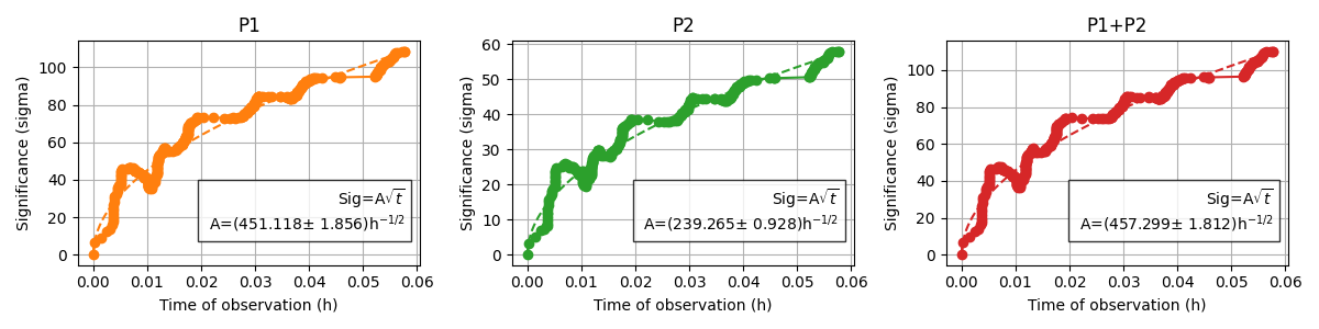
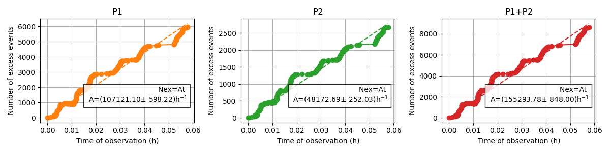
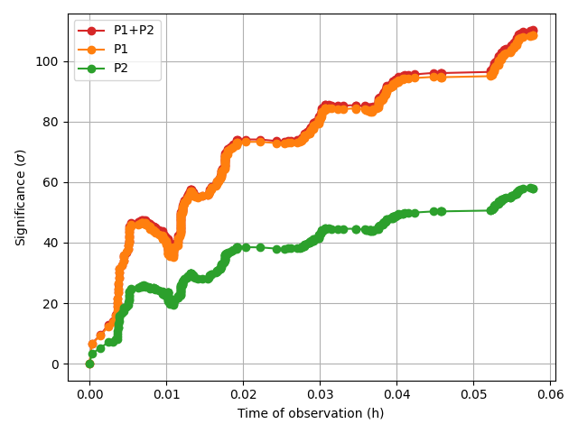
Results vs Time#
134 TimeEv = h.show_timeEvolution()
Results vs Energy#
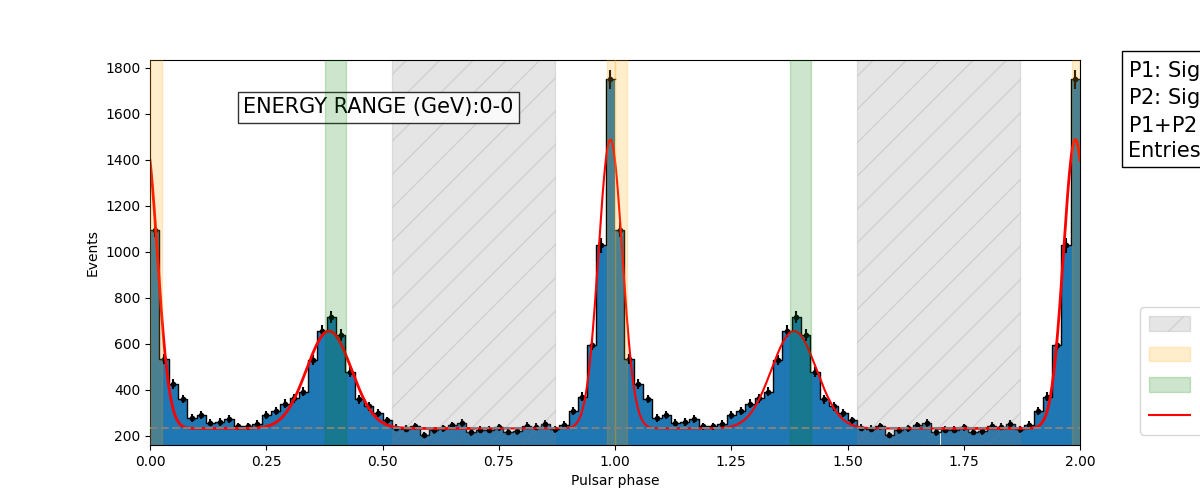
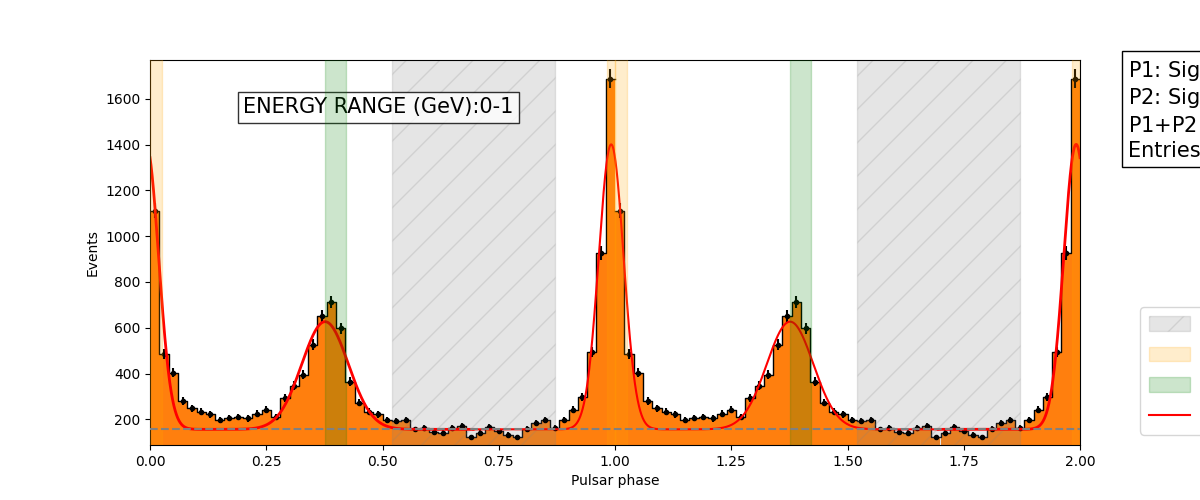
141 energy_lightcurves = h.show_lcVsEnergy()
144 energy_lc = h.show_all_lc(ylimits=None)
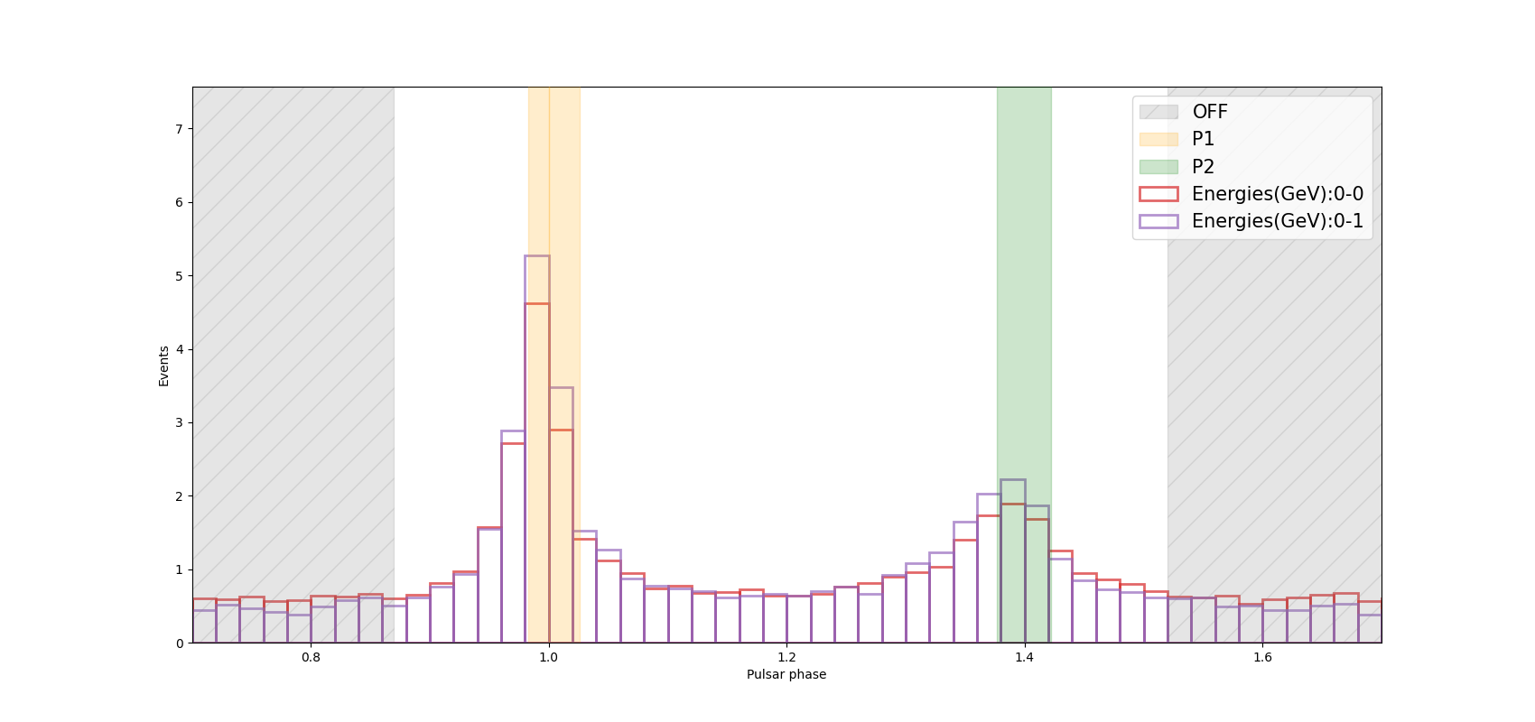
147 energy_results = h.show_EnergyPresults()
2026-10-15 10:44:16 INFO   [ptiming_ana.phaseogram.penergy_analysis] Energies(GeV): 0.1-0.316
2026-10-15 10:44:16 INFO   [ptiming_ana.phaseogram.pulsar_analysis] RESULTS FOR THE PEAK STATISTICS:
                       P1           P2        P1+P2
Significance    64.283110    32.326941    64.254439
Nex           2329.814286   994.642857  3324.457143
Nex_error       53.751332    39.787330    67.825823
Number        2828.000000  1516.000000  4344.000000
noff           498.185714   521.357143  1019.542857
sign_t_ratio     0.703795     0.353927     0.703481
s/n ratio      104.382013    43.561167   104.116125
2026-10-15 10:44:16 INFO   [ptiming_ana.phaseogram.pulsar_analysis] P1/P2 ratio=2.34 +/- 0.11
2026-10-15 10:44:16 INFO   [ptiming_ana.phaseogram.pulsar_analysis] RESULTS FOR THE PERIODICITY SEARCH:
                    Chi_square_test      Zn_test        H_test
Statistic               9894.812087  9398.711056  10117.135680
p-value                    0.000000     0.000000      0.000000
Number of $\sigma$        97.930413    96.234848     89.679481
2026-10-15 10:44:16 INFO   [ptiming_ana.phaseogram.penergy_analysis] Energies(GeV): 0.316-1
2026-10-15 10:44:16 INFO   [ptiming_ana.phaseogram.pulsar_analysis] RESULTS FOR THE PEAK STATISTICS:
                       P1           P2        P1+P2
Significance    72.157101    39.603539    73.624074
Nex           2428.965714  1109.057143  3538.022857
Nex_error       53.037924    38.897574    66.437898
Number        2771.000000  1467.000000  4238.000000
noff           342.034286   357.942857   699.977143
sign_t_ratio     0.790003     0.433594     0.806064
s/n ratio      131.336840    58.620170   133.726878
2026-10-15 10:44:16 INFO   [ptiming_ana.phaseogram.pulsar_analysis] P1/P2 ratio=2.19 +/- 0.09
2026-10-15 10:44:16 INFO   [ptiming_ana.phaseogram.pulsar_analysis] RESULTS FOR THE PERIODICITY SEARCH:
                    Chi_square_test       Zn_test        H_test
Statistic              12360.395436  11771.055229  12826.853971
p-value                    0.000000      0.000000      0.000000
Number of $\sigma$       109.750929    107.838824    100.990631
150 energy_plots = h.show_EnergyAna()
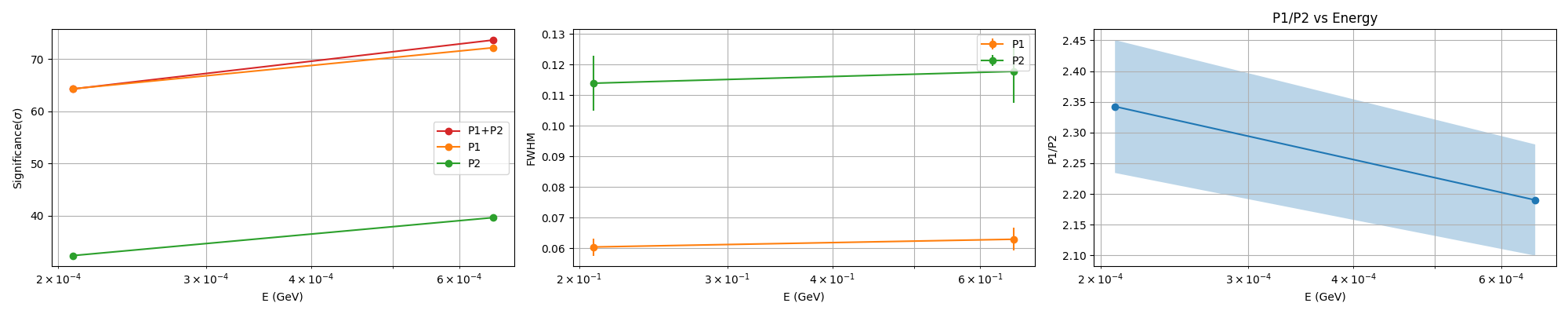
Fit vs Energy#
157 mean_energy_plot = h.show_meanVsEnergy()
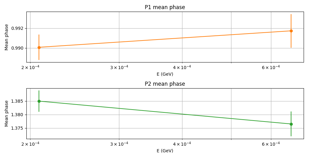
2026-10-15 10:44:17 INFO   [ptiming_ana.phaseogram.penergy_analysis] Energies(GeV): 0.1-0.316
2026-10-15 10:44:17 INFO   [ptiming_ana.phaseogram.pulsar_analysis] FITTING RESULTS:
      Name       Value     Error
0       mu    0.990064  0.001285
1    sigma    0.025658  0.001199
2     mu_2    1.384944  0.003914
3  sigma_2    0.048394  0.003781
4        A  231.375000  0.000000
5        B   80.804887  3.667207
6        C   51.361385  3.643919
2026-10-15 10:44:17 INFO   [ptiming_ana.phaseogram.penergy_analysis] Energies(GeV): 0.316-1
2026-10-15 10:44:17 INFO   [ptiming_ana.phaseogram.pulsar_analysis] FITTING RESULTS:
      Name       Value     Error
0       mu    0.991737  0.001711
1    sigma    0.026729  0.001598
2     mu_2    1.376496  0.004604
3  sigma_2    0.050032  0.004348
4        A  156.375000  0.000000
5        B   83.366327  4.920670
6        C   58.966419  4.808841
Total running time of the script: (0 minutes 14.073 seconds)